Step 1: Building a database of cognates
Cognates are similar words shared across languages and taken to indicate relatedness via common ancestry. To be diagnosed as cognate, the words must have similar meaning and, most importantly, show systematic sound correspondences indicating a common origin. For example, the English word five has cognates in German (fünf), Swedish (fem) and Dutch (vijf), reflecting descent from proto-Germanic (*fimf). Cognate identification can be tricky. For example, other cognates of these words for five include Irish cuig, Italian cinque, Armenian hing and Polish piec. In these cases, however, the sounds in the words have changed enough that they no longer look similar. It’s only by comparing words across these languages that we can detect systematic similarities, which lets us figure out that these words all go back to the same ancestral form. Conversely, known borrowings, such as English mountain from French montagne, reflect more recent contact, rather than common ancestry, and so are not treated as cognates.
The table below shows an example dataset with six languages and cognate sets colour coded across four meanings.

Because all languages change in approximately the same ways, we are able to compile similar cognate sets for Australian languages. We compiled a database of word forms and cognacy judgements for 200 meanings across 306 Pama-Nyungan languages, the oldest data coming from 1790, and the most recent from 2000. The meanings we used are basic vocabulary items – including kinship terms (mother, father), body parts (hand, ear, eye), terms for the natural world (water, fire) and basic verbs (to run, to walk, to push) – that are thought to be relatively universal and resistant to borrowing. The dataset was built up from existing sources using expert linguists to make the cognate judgements. We recorded the presence or absence of more than 18,000 sets of cognate words across the languages in our sample. The data is available from the Chirila database.
Step 2: Location data
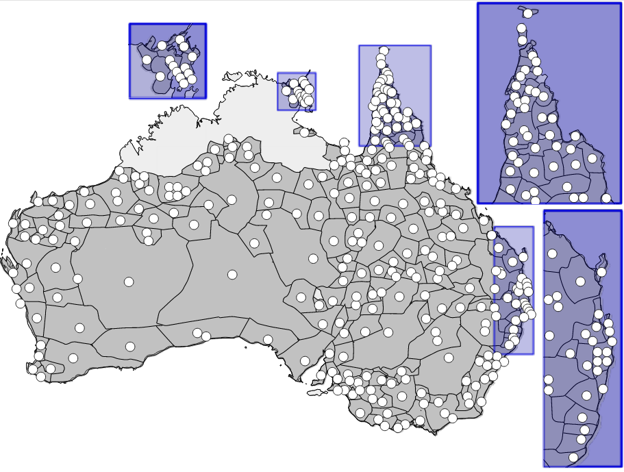
To work out where Pama-Nyungan languages have come from, we use information about where the languages in our sample are spoken today and where the extinct languages are thought to have been spoken. The figure below shows the distribution of the languages. Grey areas show the region where a language is spoken, white dots shows the approximate centroid used as point location for a language. Some languages share the same region, which is shown as multiple white dots within the same region.
Step 3: Building family trees of languages
Languages evolve through time in a manner similar to biological species. As groups of speakers become separated, their speech drifts apart forming new descendant languages, and eventually whole families of related languages. Over thousands of years this process has generated the 7000+ languages in the world today.
We can represent the relationships between languages on a family tree, otherwise known as a ‘phylogeny’. A simple example of a phylogeny is a family tree where the leaves of the tree represent the children in a family and branches represent relationships between parent and child.
Likewise, a language phylogeny shows the family tree relationships between languages. As an example from the Indo-European languages, given this is written in an Indo-European language, Dutch and Flemish are sister languages that have a very recent common ancestor. English is a cousin language, which is a bit further away from Dutch and Flemish. The Scandinavian languages are distant cousins. The points where the branches of the tree come together represent older languages that gave rise to descendents in the tree. Because all languages change in similar ways, we can use the same approach to infer ancestral relationships between the languages of Australia.

We model the evolution of Pama-Nyungan languages as the gain and loss of cognates along the branches of an unknown family tree, using an approach called Bayesian phylogenetic inference to infer the set of language trees that makes the cognate data most likely.
We explored a number of different models of cognate gain and loss, but the model that was best supported by the data was the so called ‘covarion’ model, which allows cognates to be gained and lost at intermittently fast and slow rates. It appears robust to borrowing events and usually fits cognate data reasonably well.
For more on Bayesian phylogegraphy, you can find a primer here.
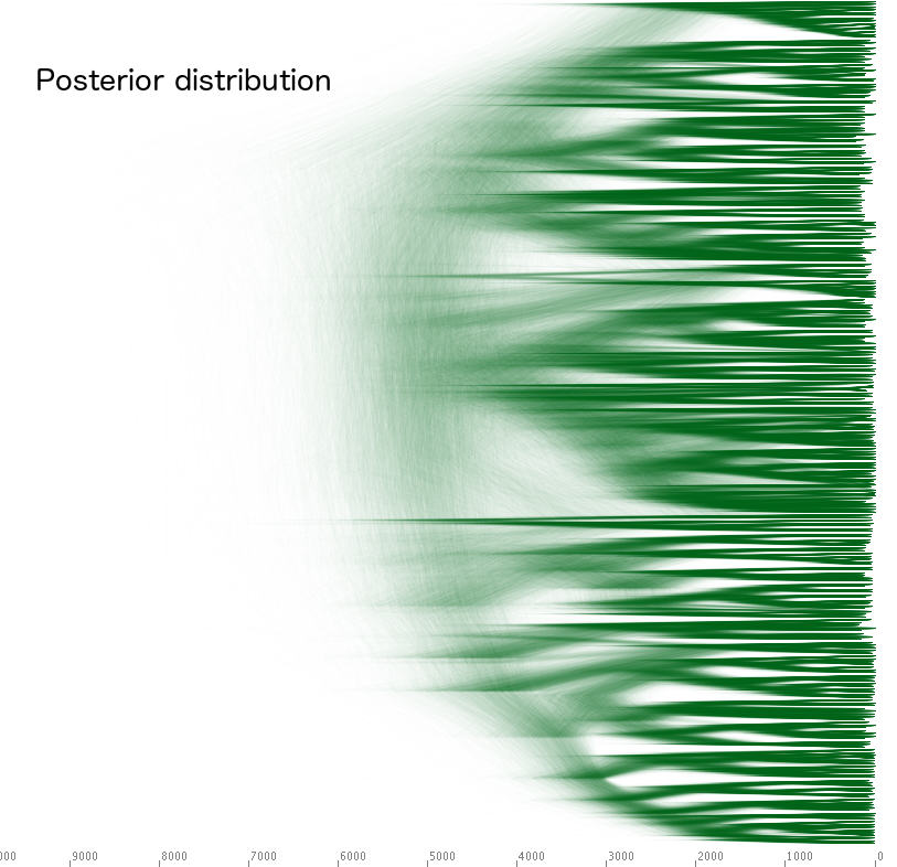
It is important to keep in mind that Bayesian methods only deal with distributions, representing the uncertainty in our knowledge. Below, you see the prior left – the state of our knowledge before we looked at the cognate data – and the posterior right – the state of our knowledge, after we incorporated the cognate data. The triangles in the prior are due to sub-family languages being constrained to group together, but there is high uncertainty with respect to the timescale and the internal branching structure of the tree. The posterior tree on the right has much less uncertainty.

Step 4: Calibrating the age of the tree
In order to provide a timescale for the expansion of the family, we need some information about how fast languages change. We do this by constraining the age of known calibration points on the tree. Unfortunately, it is not easy to find a calibration point for Pama-Nyungan languages since there are no historical documents (unlike Indo-European languages for which the written record goes back more than 3,000 years). This also makes it hard to link archeological findings to particular languages. We used archeological evidence for expansion into the well-studied Western desert region during the last 5000 years. Since only languages from the Wati-subfamily are spoken in that region, we were able to calibrate the separation of Wati languages based on the time of arrival in the Western Desert. The calibrations were chosen conservatively to span a broad age range.
There are some other potential calibration points, especially based on archeological findings on offshore islands. However, these turned out to be difficult to link with specific language splits in our tree, and were typically also very young dates, of limited use for calibrating rates across the tree. Rather than using further (potentially incorrect) calibration points, we used the more robust Wati calibration and then discuss (in the supplementary materials to the paper) how well our inferred time scale of internal diversification in the family fits findings based on the archaeological record.
It is well known that rates of language change can vary through time, so rather than assuming a strict clock-like rate of cognate gain and loss, we allowed rates to vary along the branches of the tree. The amount of variation was itself estimated from the data.
 >
>Step 5: Modelling language expansion
We combine our inferences about the Pama-Nyungan language family tree with information about where these languages are spoken (or were spoken in the case of languages which are no longer spoken). From the known locations at the ‘leaves’ of the tree, we can trace back along the branches to estimate the location at the root.
To do this, we adapt a Bayesian phylogeographic approach initially developed for tracing the origins of virus outbreaks, but rather than tracing viral lineages, we are tracing languages. The method models spatial diffusion of languages as a Brownian ‘random walk’ in two dimensions (latitude and longitude) along the branches of the tree. Put simply, this means that for a given time interval, the geographic distribution of languages expanding from some point of origin is assumed to be approximated by Brownian motion – some languages will have moved far, some will not have moved at all, but most will have moved somewhere in between. In fact, the assumptions of the model are even less restrictive because we ‘relax’ the random walk to allow the average rate of movement to vary across the tree – like with variation in rates of cognate replacement, the extent to which rates of expansion varied was estimated from our data. Note that we are not claiming that languages are viruses! This type of modeling was first used to model how viruses spread, and the same type of modeling can be used for languages.
We introduced two new ideas to make the linguistic migration process more realistic. First, the random walk models assume that at a split in the tree, the population separates and both descendents perform a random walk, moving away from each other. In the current paper, in an effort to improve model realism, we introduce a new model in which one population remains at it’s current location, whilst the second population (the founder) disperses to new territory. This ‘founder-dispersal’ model implies that at a split in the tree a random walk happens on only one of the two branches that appears, while the other remains in the same place. An small-scale analogy is when children grow up and move out of home, it does not imply that the parents also move.

Second, to allow for variation in rates of movement due to features of the landscape, instead of performing a random walk over a two dimensional space, we perform a random walk over a grid, where the probability of moving to a neighbour depends on the landscape. For example, in the figure below any point on the grid near water – including areas near the Murray Darling river system – are assigned a different rate than those in the interior. Grid points that fall in water are excluded, since no extensive seafaring activities have been known for Indigenous people in this region. For simplicity, we modeled only major waterways, not every river system.

Step 6: Testing between the hypotheses
The Bayesian approach we employ means that we can directly compare support for each of the four main hypotheses. This is because the method we use does not produce a single answer – e.g. the origin is at x degrees longitude and y degrees latitude. That would not be all that useful, because if you want to test between competing theories, you need some estimate of uncertainty – how sure are you that the origin is at one location versus another?
There is uncertainty in the relationships between the Pama-Nyungan languages (nobody can say with absolute certainty that one particular family tree is the true one – for 100 languages there are already more possible trees than there are atoms in the universe!), there is uncertainty in the time scale (we can’t know for sure exactly how fast languages change), and even if we knew the family tree and time scale exactly, there is uncertainty in the geographic expansion process so we cannot pin down the location of the root exactly.
One of the major advantages of the Bayesian approach is that we do not produce a single answer, but instead account for all those uncertainties using some clever algorithms (called Markov Chain Monte Carlo methods) that sample language trees, divergences times and locations at all points on the tree, in proportion to how likely they make our observed data. In terms of the origin location, if an origin is twice as likely, and we do not prefer any location over any other a priori, then we should see it twice as often in our sample.
So we were able to run our analyses and directly compare how often the origin locations we inferred fell in the range proposed for the four hypotheses. As we report in the paper,
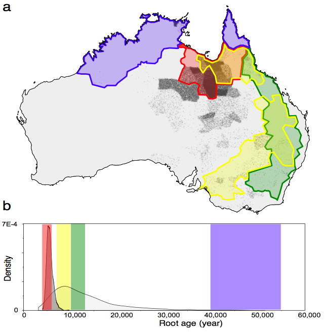
hypothesis 1 – a recent origin of Pama-Nyungan originating south of the Gulf of Carpentaria – was strongly supported.
You can see this visually in our Figure 1, below. Most of the points fall in the rapid replacement (red – H1) area, and there is some support for the early Holocene (yellow – H2) hypothesis, but very little support for post ACR (green – H3) and none for initial colonisation (blue – H4) hypothesis. Together with the timing of the root age shown below, our analysis finds that the origin of H1 is orders of magnitude more likely than any of the other hypotheses.